A Neural Network to Detect Thin hBN Layers on Wafers
Introduction
During my undergraduate research at the University of California, Berkeley (Sep 2023 - Jan 2024), I worked on Charge Transfer Dynamics in RuCl₃/hBN/WSe₂ Heterostructures under Professor Feng Wang. To enhance experimental efficiency, I independently developed a Convolutional Neural Network (CNN) that detects thin hBN layers on wafers with 95% accuracy.
Project Motivation
The current flake finding system used in laboratories cannot effectively handle thin hBN because thin hBN, wafers, and residue on tape often have similar colors. Traditional color-based algorithms frequently misidentify residue as flakes, causing significant inefficiencies as researchers need to spend considerable time distinguishing between residue and actual flakes. This inefficiency has prompted the integration of machine learning techniques for improved accuracy and efficiency.
Neural Network Architecture
The developed CNN architecture is both simple and effective. Below is the structure implemented:
1
2
3
4
5
6
7
8
9
10
11
12
13
14
15
16
17
18
19
20
21
22
23
24
25
import torch
import torch.nn as nn
import torch.nn.functional as F

class Net(nn.Module):
    def __init__(self):
        super().__init__()
        self.conv1 = nn.Conv2d(3, 6, 5)  # Output: 6 channels, 59x59 feature maps
        self.pool = nn.MaxPool2d(2, 2)
        self.conv2 = nn.Conv2d(6, 16, 5)  # Output: 16 channels, 13x13 feature maps
        self.fc1 = nn.Linear(16 * 13 * 13 , 64)
        self.fc2 = nn.Linear(64, 32)
        self.fc3 = nn.Linear(32, 2)  # Output: 2 classes (Sample, Tape)

    def forward(self, x):
        x = self.pool(F.relu(self.conv1(x)))
        x = self.pool(F.relu(self.conv2(x)))
        x = torch.flatten(x, 1)  # Flatten all dimensions except batch
        x = F.relu(self.fc1(x))
        x = F.relu(self.fc2(x))
        x = self.fc3(x)
        return x

net = Net()
net.to(device)
Dataset and Preprocessing
The dataset comprised approximately 50,000 images, manually labeled as tape or flake, with flake images constituting about 2% of the dataset.
Preprocessing Steps:
Color Normalization: Adjusting the images based on wafer color standards to account for color variation in wafers scanned at different times. The standardization result is shown below.
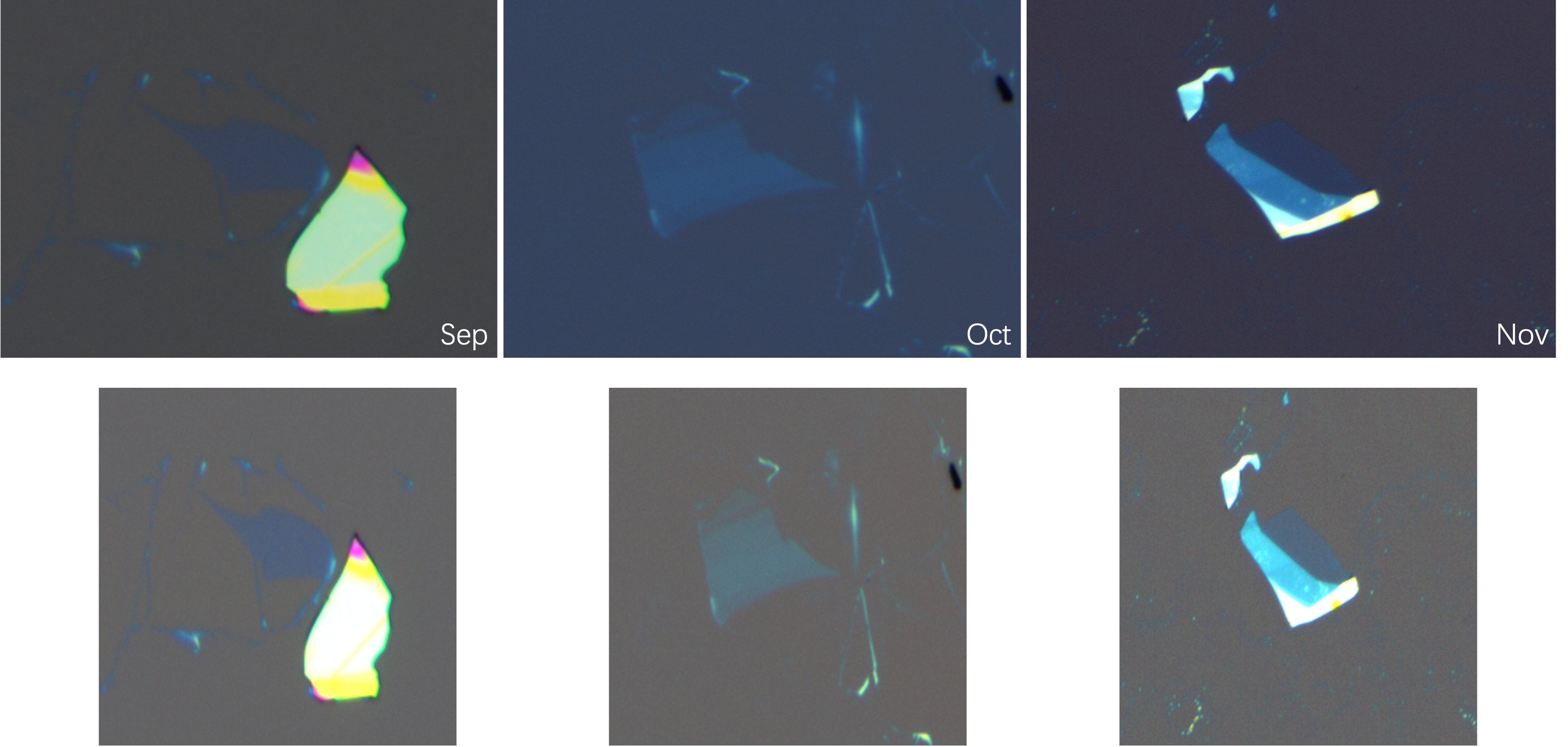 Color variation in wafers scanned at different months and the standardized result after applying color normalization
- Standard Transformations:
- Scaling
- Type Conversion
- Normalization
- Data Augmentation for Flake Images:
- Rotation
- Symmetry Transformations
- Scaling
These methods helped enhance the dataset, particularly augmenting the minority flake class for better model training.
Training and Testing
The training process involved splitting the dataset, with 10% reserved as a validation set. Following are the results after 400 epochs of training:
1
[Epoch 396/400] [Loss: 19.741972] [Acc: T_S: 99.32% T_T: 95.51% V_S: 94.95% V_T: 94.71%] [Time: 109.3]
Accuracy Metrics:
- T_S (Sample): Training set accuracy for Sample (flake)
- T_T (Tape): Training set accuracy for Tape
- V_S (Sample): Validation set accuracy for Sample (flake)
- V_T (Tape): Validation set accuracy for Tape
The following sections highlight the model performance at different learning rates and epoch counts:
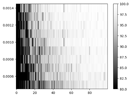 Accuracy of Sample identification (flake) at different learning rates and epochs.
 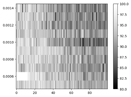 Accuracy of Tape identification at different learning rates and epochs
 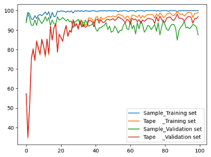 Accuracy at learning rate 0.0007 over epochs.
Results and Visualizations
The validation set’s weight distributions and samples correctly/incorrectly identified by the model are illustrated below:
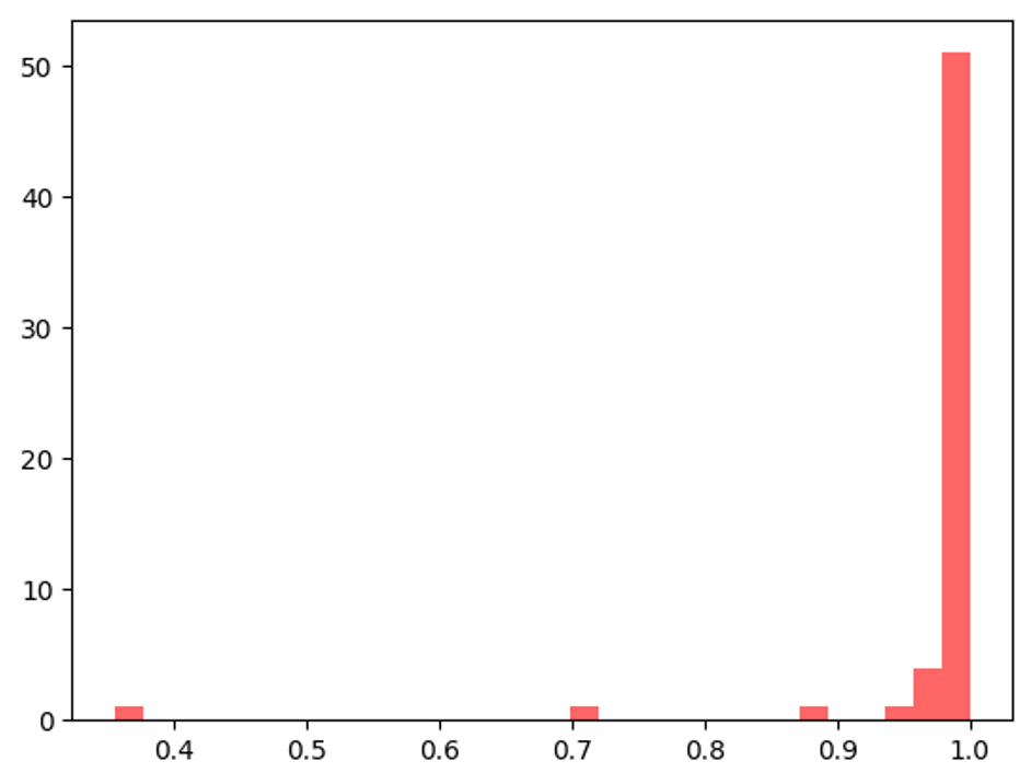 Weight Distribution of Sample (flake)
 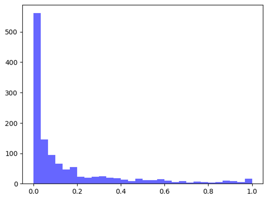 Weight Distribution of Tape
 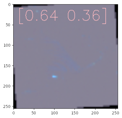 Incorrectly Identified Samples (flake)
 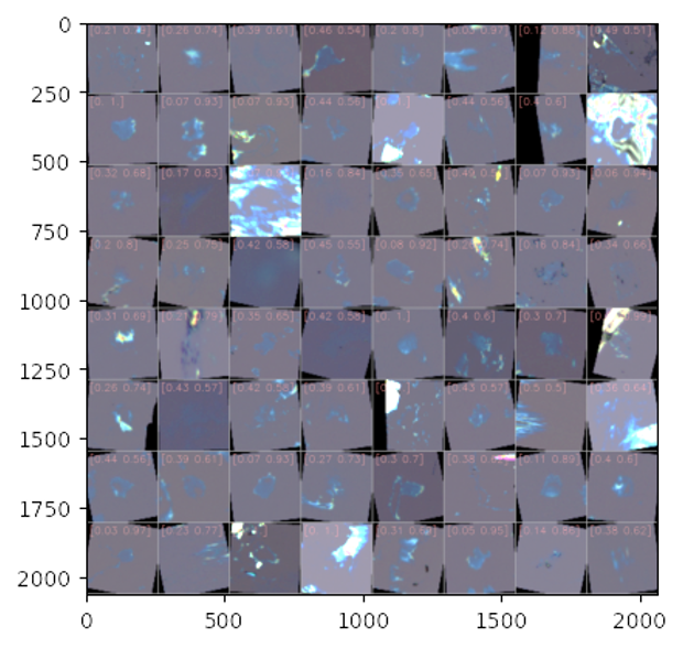 Incorrectly Identified Tape