Investigating Propagation Dynamics of Truncated Vector Vortex Beams -- A Simulation Study

1. Introduction

As a second-year physics student at Xi’an Jiaotong University, I had the opportunity to get some research training under the supervision of Professor Hong Gao. Our work focused on replicating the theoretical calculations and simulations presented in the paper “Investigation of Propagation Dynamics of Truncated Vector Vortex Beams” by P. Srinivas et al. This blog post summarizes my research experience and the key findings from our simulation study.

---

2. Simulation Methodology

We developed a MATLAB program to simulate the propagation of truncated vector vortex beams. The key steps in our simulation include:

1. Generating the input Gaussian beam with a specific orbital angular momentum.
2. Applying spatial truncation to create the truncated vector vortex beam.
3. Implementing phase modulation to simulate focusing.
4. Using the angular spectrum method to propagate the beam through space.
5. Analyzing the resulting intensity distributions and polarization states at different propagation distances.

Our simulation allowed us to investigate various configurations, including different orbital angular momentum values and truncation patterns.

function [x,y,xInput,yInput,x2,y2] = Main(typea,typeb,d)
%MAIN Summary of this function goes here
%   Detailed explanation goes here

%% Generate the input Gaussian beam
mm=1e-3;
nm=1e-9;
lambda=532*nm;% wavelength
k=2*pi/lambda;% wavevector
SL=10.24*1*mm ;% Side length
N=513;% samples for side length
dx=SL/N;%sample interval
d=d*mm;% The distance between the input and output planes
x = -0.5*SL:dx:0.5*SL-dx;% coordinate
y = x;
[X,Y]=meshgrid(x,y);
l=5;
load("HG.mat");
% T=0.3*2*pi;
% X0=abs(I0).*exp(1i*l*angle(X+1i*Y)).*exp(1i*T).*1;
% Y0=abs(I0).*exp(1i*l*angle(X+1i*Y)).*exp(1i*T).*1i;
% quiver(real(X0([1:10:end],[1:10:end])),real(Y0([1:10:end],[1:10:end])));
% axis square;
switch typea
    case 1
        xInput=abs(I0).*exp(1i*l*angle(X+1i*Y)).*1;
        yInput=abs(I0).*exp(1i*l*angle(X+1i*Y)).*1i;
    case 2
        xInput=abs(I0).*exp(-1i*l*angle(X+1i*Y)).*1;
        yInput=abs(I0).*exp(-1i*l*angle(X+1i*Y)).*(-1i);
    case 3
        xInput=abs(I0).*exp(1i*l*angle(X+1i*Y)).*1;
        yInput=abs(I0).*exp(1i*l*angle(X+1i*Y)).*1i;
        xInput=xInput+abs(I0).*exp(-1i*l*angle(X+1i*Y)).*1;
        yInput=yInput+abs(I0).*exp(-1i*l*angle(X+1i*Y)).*(-1i);
end

if typeb==0
    for ii=1:513
        for jj=1:513
            if ii>256&&jj>256
                xInput(ii,jj)=0;
                yInput(ii,jj)=0;
            end      
        end
    end
end
%% Plot Input Beam
% for Ti=1:20
%     T=Ti/10*pi;
%     x0(:,:,Ti)=xInput.*exp(1i*T);
%     y0(:,:,Ti)=yInput.*exp(1i*T);
% end
% figure; hold on; axis square;
% for xi=-0.5*SL:dx*20:0.5*SL-dx
%     for yi=-0.5*SL:dx*20:0.5*SL-dx
%         xtmp=xi+0.0005*real(reshape(x0(round((xi+0.5*SL)/dx+1),round((yi+0.5*SL)/dx+1),:),[],1));
%         ytmp=yi+0.0005*real(reshape(y0(round((xi+0.5*SL)/dx+1),round((yi+0.5*SL)/dx+1),:),[],1));
%         plot(xtmp,ytmp,'k');
%     end
% end

%% Phase moduation to focus
OPD = 3*mm;
f=200*mm;
P_input = exp(-1i*k/(2*f)*(X.^2+Y.^2));
% figure;mesh(X,Y,1/(2*f)*(X.^2+Y.^2));
% title('Surface of lens');
% xlabel('x(m)');
% ylabel('y(m)');
% zlabel('t(m)');
x1=xInput.*P_input;
y1=yInput.*P_input;

%% Gaussian Beam

% I_input=exp(-2*((X /(0.5* SL)).^2+(Y/(0.5* SL)).^2)); %The input Gaussian beam
% %load("U1.mat")
% % I0=InputGeneration(N);
% % save("HGData1.mat","I0");
% load("HGData1.mat");
% for ii=1:513
%     for jj=1:513
%         if ii>128&&ii<385&&jj>128&&jj<385
%             I1(ii,jj)=I0((ii-128)*2,(jj-128)*2);
%         else
%             I1(ii,jj)=0;
%         end      
%     end
% end
% 
% I_input=abs(I1);
% figure;
% pcolor(x,y,abs(I_input));
% axis square;
% shading interp; 
% xlabel('x(m)');
% ylabel('y(m)');
% colorbar;colormap("gray");
% title('Amplitude of Gaussian beam');


%% Angular spectrum
fx=-1/(2*dx):1/SL:1/(2*dx)-1/SL;  %freq coords
[FX,FY]=meshgrid(fx,fx);
H=exp(1i*k*d*sqrt(1-(lambda*FX).^2-(lambda*FY).^2));  %trans func
H=fftshift(H);
X1=fft2(fftshift(x1));  %shift.fft source filed
X2=H.*X1;    %multiply
x2=fftshift(ifft2(X2));

Y1=fft2(fftshift(y1));  %shift.fft source filed
Y2=H.*Y1;    %multiply
y2=fftshift(ifft2(Y2));


%% Plot Output Beam
% for Ti=1:20
%     T=Ti/10*pi;
%     x0(:,:,Ti)=x2.*exp(1i*T);
%     y0(:,:,Ti)=y2.*exp(1i*T);
% end
% figure; hold on; axis square;
% nn=0.0003;
% for xi=-0.5*SL:dx*20:0.5*SL-dx
%     for yi=-0.5*SL:dx*20:0.5*SL-dx
%         xtmp=xi+nn*real(reshape(x0(round((xi+0.5*SL)/dx+1),round((yi+0.5*SL)/dx+1),:),[],1));
%         ytmp=yi+nn*real(reshape(y0(round((xi+0.5*SL)/dx+1),round((yi+0.5*SL)/dx+1),:),[],1));
%         plot(xtmp,ytmp,'k');
%     end
% end

%% Tmp
% Tmp=y2;
% pcolor(x,y,abs(Tmp));
% axis square;
% shading interp; 
% xlabel('x(m)');
% ylabel('y(m)');
% colorbar;colormap("gray");
% title('Amplitude of Gaussian beam');
% figure;
% pcolor(x,y,angle(Tmp));
% axis square;
% shading interp; 
% xlabel('x(m)');
% ylabel('y(m)');
% colorbar;colormap("gray");
% title('Amplitude of Gaussian beam');
end

---

3. Results and Discussion

Our simulations produced two main types of results:

1. Energy distribution maps: These show how the intensity of the beam changes as it propagates. We observed that the truncated vector vortex beam tends to “heal” itself within the Rayleigh range, temporarily regaining a structure similar to an untruncated beam. In the far field, the truncated portion reappears, but rotated 180 degrees from its original position.

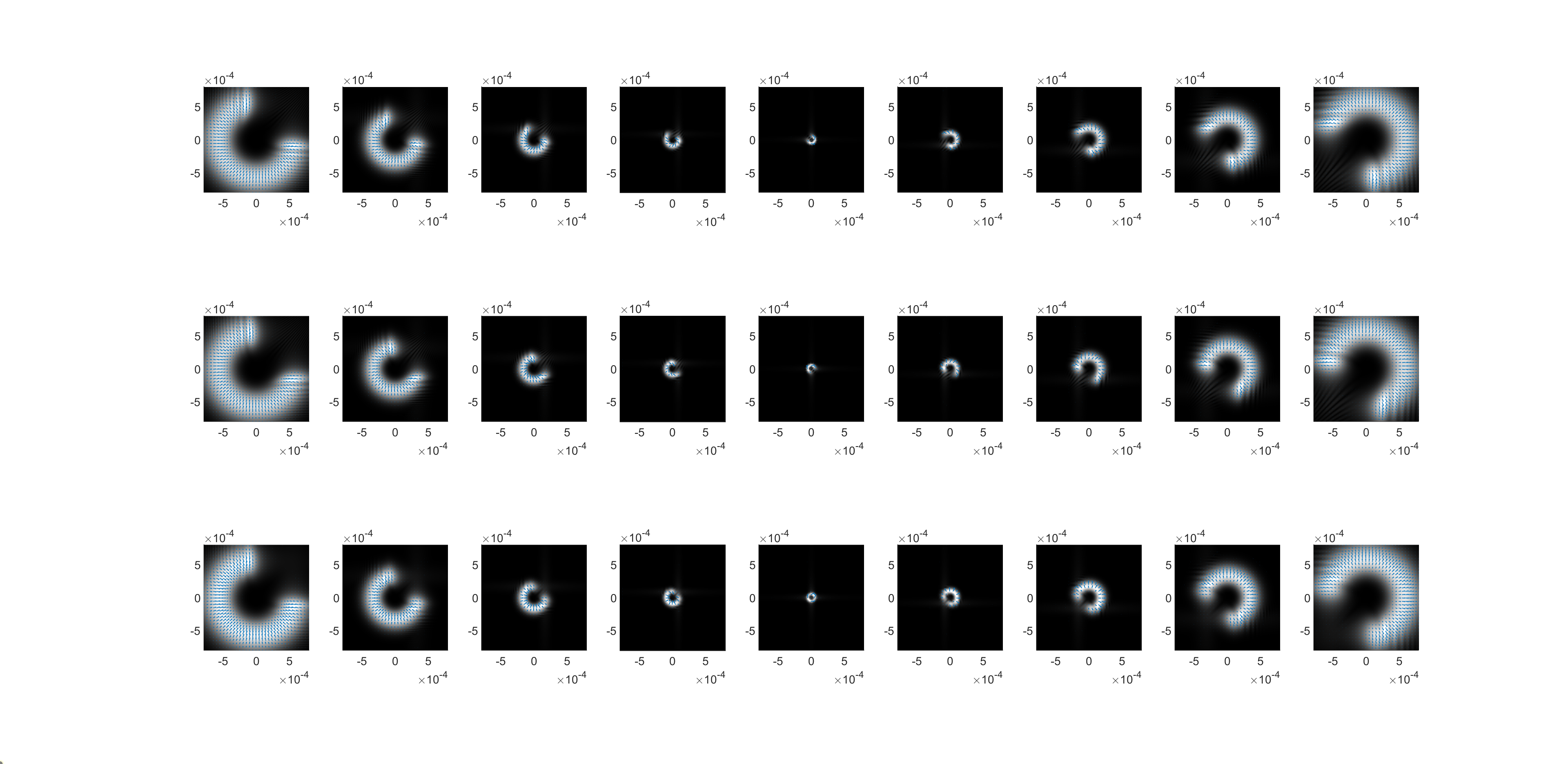Energy Distribution

1. Polarization state distributions: These maps illustrate how the polarization of the beam evolves during propagation. Interestingly, we found that the overall polarization structure of the composite beam is largely preserved along the propagation axis, despite the complex dynamics of the individual components.

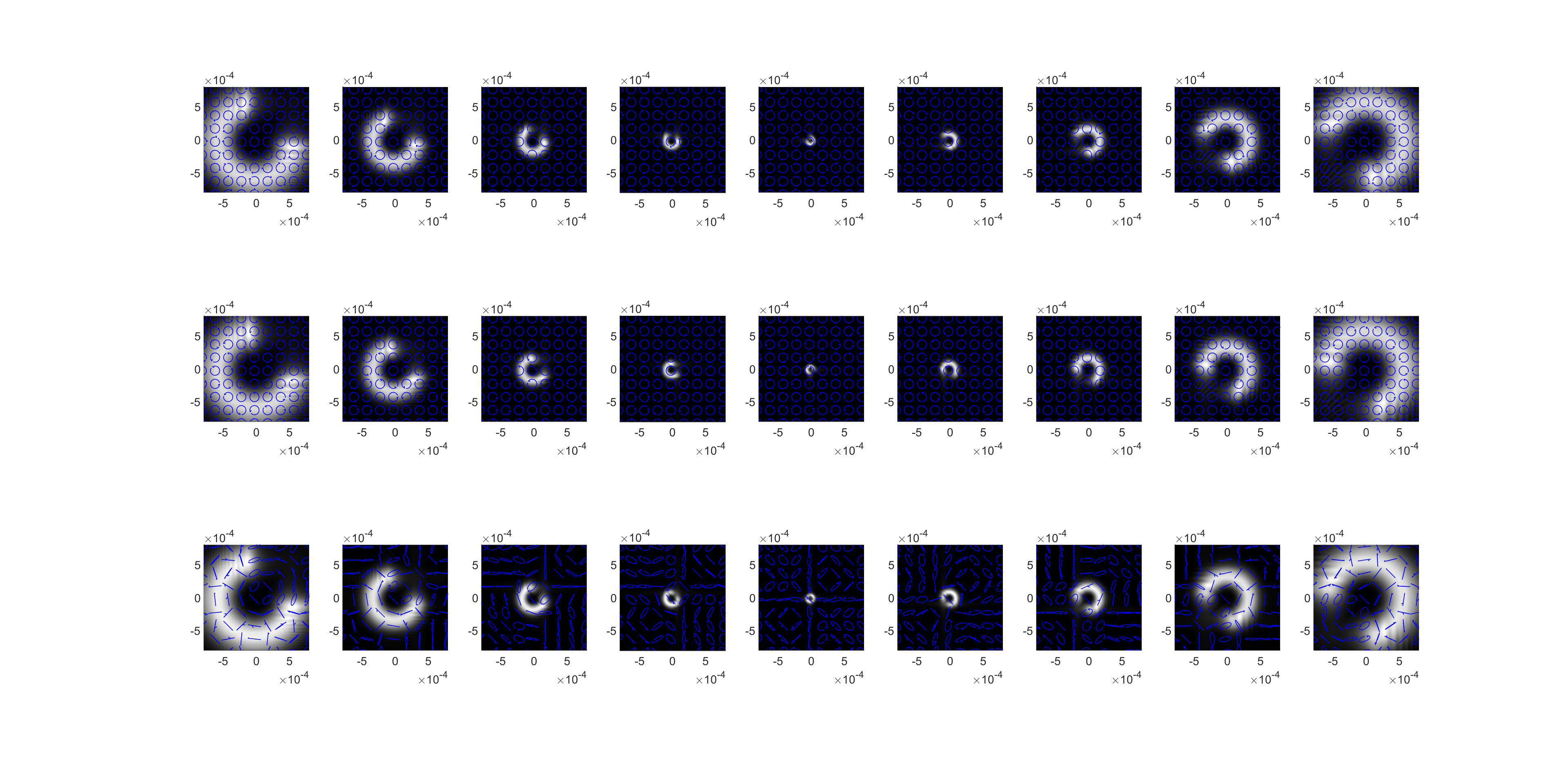Polarization Distribution

These results closely match the experimental observations and theoretical predictions described in the original paper. They demonstrate the complex interplay between the beam’s spatial structure, polarization, and propagation dynamics.

---

4. Conclusion

This research experience has provided me with valuable insights into the field of optical physics and enhanced my skills in numerical simulation and data analysis. The study of truncated vector vortex beams reveals fascinating phenomena that arise from the interaction between spatial, polarization, and propagation effects in complex optical fields.

---